I’ve been playing with calculating the entropy of a toy system used to illustrate the connection between “disorder” and entropy. (See Entropy 101 and Entropy 102.) I needed to calculate the minimum number of moves required to sort a disordered collection, but that turns out to be an NP problem (no doubt related to Traveling Salesman).

The illustration bridges Boltzmann and Shannon entropy, which got me playing around with the latter, and that led to some practical results. This article describes the code I used mainly as an excuse to try embedding my own colorized source code blocks.

I’m not going to get into entropy here (I’ve posted about it plenty elsewhere). What matters is that this code involves Shannon entropy, not Boltzmann entropy. They’re closely related but involve quite different domains and enough differences to make calling them the same thing ever so slightly questionable.

Regardless, rather than Boltzmann’s famous thermodynamic formula:

The code here uses Shannon’s version:

Which gives an answer in binary bits because of the log2 function. Using the log10 function gives a result in terms of decimal digits. The symbol density determines the log base (or vice versa).

Implementing the equation is very simple:

It can be done in a single line lambda expression if one doesn’t mind calling the probability function twice:

But I do, so first I generate a list of all the probabilities for each system micro-state (line #6). As a safety check, in the next line, I also generate a sum of those probabilities (something the one-liner can’t do). The expected sum is 1.000 (give or take a floating-point error).

Then I generate a list of summation terms (line #9), sum them to derive the entropy (line #10), and return the entropy, the total probability, and both lists. Most applications will only care about the entropy value, but the other data is available if wanted.

When run with the 27-pattern default, the demo prints:

4.754887502163471
0.9999999999999993

Telling us the entropy is ~4.755 bits and, as expected, the probabilities do sum to 1.000, give or take a floating-point error. The entropy value is the same as:

That’s because the probability function (line #15) assigns equal probability (1/NP) to all possible patterns. When all patterns are the same, the entropy is maximum and the same as the number of bits required to express all possible patterns. (If we had 32 patterns, the max entropy would be exactly 5.000 because five bits can express exactly 32 patterns.)

Note that if we change logbase to 10, then the demo prints:

1.4313637641589871
0.9999999999999993

Telling us the same 27-pattern system, when all patterns are equal, has an entropy of ~1.43 decimal digits. Setting logbase to other values results in different entropy values. The entropy just says how many symbols are required to express NP many values.

§

In a way, that’s it, everything else is an application of that calculation. But there are some interesting things we can do to explore its consequences.

Imagine we have a “tea” variable that can specify one of 27 types of tea. (Imagine a tiny dial with a pointer.) As just shown, when all 27 teas are equally likely, the dial could point to any of them, we say the variable has maximum entropy (of ~4.755 if we mean bits). This effectively means the variable is random — it has maximum surprise. Things get more interesting when we vary the pattern probabilities.

A very simple extension assigns a high probability to one pattern (tea) and a low probability to all others. We’re saying the tea dial is very likely to point to some given tea, and very unlikely to point to any other. In this simple case we’ll assign the same low probability to all other possible teas. Here’s some code:

The sum of all probabilities must be 1.000, so the probability function must be normalized. That’s why the example above used 1/NP for each pattern’s probability. The sum is NP×(1/NP), which is obviously one. Here, normalization is ever so slightly trickier.

Firstly, the demo function takes NB (number of bits), rather than NP (number of patterns). For these demos we’ll use whole numbers of bits because fractional values, such as for 27 teas, don’t really change anything. The convenience is that in using whole bits, our maximum entropy is always the number of bits.

We do need NP, so line #5 calculates it. The next line sets PF to the input argument p_of_x (probability of X) if it was provided, otherwise uses the default 1/NP (which will result in maximum entropy). We set PX to some random pattern, and line #8 defines the probability function: return PF if the pattern matches PX otherwise return a low probability calculated as 1.0-PF divided among all other patterns.

When run with defaults, the demo prints:

NB=5, NP=32
P(PX)=PF=0.031250000000
tot-prob=1.000000000000
entropy=5.000000000000

As expected, the entropy is 5.00 and the probabilities sum to 1.00. The probability of the expected number is only 3.125% — or odds of exactly 1/32 for each pattern. Maximum entropy, maximum surprise.

But if we set p_of_x=0.99, it prints:

NB=5, NP=32
P(PX)=PF=0.990000000000
tot-prob=1.000000000000
entropy=0.130335099000

A much-reduced entropy value. There is a 99% probability the dial will point to the expected number, so there is very little surprise. We can take things even further by setting p_of_x=0.999999 — a near certainty of the expected answer:

NB=5, NP=32
P(PX)=PF=0.999999000000
tot-prob=1.000000000000
entropy=0.000026328459

Almost no surprise at all.

§

Looking at the way making one answer more likely changes the entropy naturally led me to charting the curve as entropy is reduced this way from maximum to some tiny value. (It approaches zero, but since log(0) is an invalid expression, it can never get there.)

Here’s some code:

It starts off like the demo above, but line #12 calculates a list of probabilities from 1/NP to (NP-1)/NP — which approaches, but doesn’t reach, 1.00. Two extra probabilities getting even closer to 1.00 get tacked on to get the curve closer to zero.

When run it prints a list:

   1: 0.031250000 = 5.000000000000 (1.000000)
   2: 0.062500000 = 4.981849107605 (1.000000)
…
…
  32: 0.999999000 = 0.000026328459 (1.000000)
  33: 0.999999900 = 0.000002965039 (1.000000)

I used a function like this to generate data I could make a chart with:

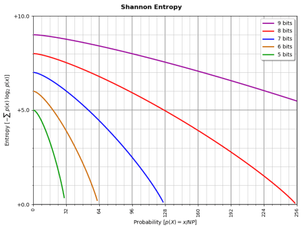
As you see, the entropy curve approaches zero. Mathematically it can’t get there, but conceptually, if the probability is 1.00, there’s no surprise in the answer (effectively, it’s already known) and the entropy is zero.

§

This post was mainly an excuse to see if inserting my HTML Python code would work (look like). I’ll leave you with a complete class you can use for your own explorations:

I won’t explain it here unless someone expresses an interest.

Ø