This series of posts is for those who have used a programming language before but are not familiar with Python. The first six posts introduced the language, and the seventh discussed downloading, installing, and using it.

The previous two posts (see part 8 and part 9) explored creating classes (aka data types) in Python. This post wraps up that exploration (for now).

In the last two posts we implemented for our 3D Point class:

1. The data attributes x, y, and z.
2. A constructor method with x, y, and z parameters.
3. String representations for both str and repr contexts.
4. A Boolean True/False value.
5. A full list-like interface for iteration and indexed access.
6. The ability to do math with points (add, subtract, multiply, divide).

To wrap things up, we’ll add some custom methods to implement common things we might do when working with 3D points.

First, let’s demonstrate and exercise the math abilities of our point objects:

When run, this prints:

[0.500, 0.250, 0.125]
[1.000, 1.000, 1.000]

Point Math:
p1 + p2 = [1.500, 1.250, 1.125]
p1 - p2 = [-0.500, -0.750, -0.875]
p1 * p2 = [0.500, 0.250, 0.125]
p1 / p2 = [0.500, 0.250, 0.125]

Scalar Math:
p1 + 1.0 = [1.500, 1.250, 1.125]
p2 - 0.5 = [0.500, 0.500, 0.500]
p1 * 2.0 = [1.000, 0.500, 0.250]
p1 / 0.5 = [1.000, 0.500, 0.250]

1.0 + p1 = [1.500, 1.250, 1.125]
0.5 - p2 = [-0.500, -0.500, -0.500]
2.0 * p1 = [1.000, 0.500, 0.250]
0.5 / p1 = [1.000, 2.000, 4.000]

Inplace Point Math:
p0=[0.000, 0.000, 0.000]
p0 += p1 ⇒ p0=[0.500, 0.250, 0.125]
p0 -= p2 ⇒ p0=[-0.500, -0.750, -0.875]
p0 *= p1 ⇒ p0=[-0.250, -0.188, -0.109]
p0 /= p1 ⇒ p0=[-0.500, -0.750, -0.875]

Inplace Scalar Math:
p0=[0.000, 0.000, 0.000]
p0 += 0.50 ⇒ p0=[0.500, 0.500, 0.500]
p0 -= 0.25 ⇒ p0=[0.250, 0.250, 0.250]
p0 *= 3 ⇒ p0=[0.750, 0.750, 0.750]
p0 /= 3 ⇒ p0=[0.250, 0.250, 0.250]

Which are all expected results, so the math checks out.

If we’re doing math with points, we might also need to compare two points to see if they are equal or not. As with the math operators, there are dunder methods for the equality operators:

Lines #8 to #21 implement the dunder eq method (“equals”), which Python calls when objects are compared with ==, the equality operator.

As with most operator methods, the method takes two parameters: self and other (representing the left and right sides of the operation respectively). The former is always a Point object, but as we saw in the math methods, other can potentially be any object. That’s why lines #12 and #13 test to see of other is the same type as self and raise an Exception if it isn’t.

Equality between two points requires that all three elements match, so lines #16 to #18 test each pair of elements and return False on a mismatch. If all three tests succeed, the points are equal, and we fall through to line #21 and return True.

Lines #23 to #25 implement the dunder ne method (“not equals”), which Python calls when objects are compared with !=, the inequality operator.

Since inequality is the opposite of equality, we just call dunder eq and return its negation.

Note that Python has two ways of comparing objects:

Firstly, there are the equality and inequality operators, == and !=. These compare the values of objects. For instance, ((3+4) == 7) has a Boolean True value and so does ((2+2) != 5). So, lines #10 and #17 both invoke the dunder eq method, and #11 and #18 both invoke the dunder ne method.

Lines #21 to #28 exercise Python’s other comparison test, the is operator, which compares based on the two objects identity (typically, their address in memory).

When run, this prints:

[1.000, 2.000, 3.000] @01f5bf1b2900
[1.000, 2.000, 3.000] @01f5bf29c050

p1 == p2 = True
p1 != p2 = False

p1 == p2 = False
p1 != p2 = True

p1 is p1 = True
p1 is p2 = False

p1 is not p1 = False
p1 is not p2 = True

It may seem trivial in this example that (p1 is p1) and (p1 is not p2), but consider this example:

When run, this prints:

[1.000, 2.000, 3.000] @021069432900
[1.000, 2.000, 3.000] @021069432900

p1 == p2 = True (of course)
p1 is p2 = True (same object)

function: p is p1 = True (same object)
function: p is p1 = True (same object)

In the code above, there is only ever one Point object, the one created on line #3. We create an alias, named p2, on line #4, and it refers to the same object.

Importantly, when we pass an object to a function, we pass a reference to it. (And remember that methods are functions.) This means a function can modify a passed object if that object is mutable:

When run, this prints:

[1.000, 1.000, 1.000]
[3.000, 4.000, 5.000]

The bottom line is that we need to be aware of when objects are actually created and when there are references to existing objects.

When we create new points, we can provide their x, y, and z values, but once we have a one, we can only change its values one at a time. It might be nice to have a way to change all three elements with one call. Effectively, we want to move the point from one coordinate to another:

Lines #8 to #13 implement the reset method, which sets all elements to zero (geometrically, it moves the point to the origin).

Lines #15 to #20 implement the move method. In addition to self, it takes three additional parameters: x, y, and z. These all have default values, which makes them optional — callers can supply them or not and in any order.

We use a default value of None to allow us to detect whether the parameter was passed. (The assumption is that None isn’t a valid input value. All possible numeric inputs are valid, so we can’t use, for instance, zero or minus one.) We only change the object properties if the parameter is not None. This lets callers change any or all values:

When run, this prints:

after move: [2.700, 3.100, 5.500]
after reset: [0.000, 0.000, 0.000]
after move: [0.000, 4.200, 0.000]
after move: [0.000, 3.142, 6.300]
after move: [2.100, 3.142, 6.300]
after move: [1.000, 2.000, 3.000]

Note that, when no keywords are provided (line #18 and #21), Python fills in the arguments positionally (as defined in the method). So, line #18 provides a new value for the x element, and line #21 provides all three in x, y, z order.

It’s not uncommon to use points as vectors — as “arrows” with their tails at the [0,0,0] coordinate (aka the origin) and their tips at the point determined by their [x,y,z] coordinate.

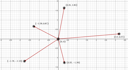
This is true in any dimension, so 2D points represent 2D vectors, 3D points (such as our Point class) represent 3D vectors, and so on for however many dimensions. The key difference between points and vectors is that vectors have a direction in which they point and a size or magnitude.

The point/vector distinction is largely in how the objects are used, but we can add some methods to implement some common vector operations.

An obvious one, given the definition of a vector as an “arrow”, is the length (aka magnitude) of the vector — the distance from the origin to the point. We assume our vectors live in Euclidean space where the Euclidean distance between any two points is a generalization of the Pythagorean theorem:

When measuring from the origin, the second point is all zeros, so the length of a vector reduces to:

Let’s add a custom method to our Point class to implement vector length:

Lines #9 to #15 define a method called magnitude. Note the decorator on line #9 that begins the definition (a decorator is an at-sign followed by a name). Python decorators are an advanced topic for later, but for now think of them as modifiers of the definition that follows them.

In this case, the built-in @property decorator modifies the magnitude method to act like an attribute (aka property) rather than a method:

Note the lack of parentheses when accessing the magnitude property (lines #7 to #9 and #14). It acts like a data attribute (similar to the x, y, and z attributes). But as line #14 illustrates, it is a read-only attribute. Note also that we cannot pass arguments to a property — the method can only have the usual self parameter.

[If you want to explore decorators in detail, see Python Decorators, part 1 and part 2, as well as the redux and more follow-up posts.]

When run, this prints:

p0.magnitude = 0.0
p1.magnitude = 1.7320508075688772
p2.magnitude = 7.857480512225276

Trying to change magnitude:
OOPS: AttributeError
property 'magnitude' of 'Point' object has no setter

The error message text is a clue to an important (but advanced) Python rabbit hole that likely goes beyond this series. [If interested in the details, see Python Descriptors, part 1 and part 2.]

The Point code above includes a normalized method (lines #17 to #28) that also uses the @property decorator to convert it to a read-only attribute. This method returns a new vector that points in the same direction but has a length of one. In many vector operations we care about the direction but not the magnitude. In fact, we generally want the magnitude to be one — normalized vectors are useful in vector calculations.

Let’s exercise the normalized property:

When run, this prints:

p0.magnitude = 0.0
p1.magnitude = 1.7320508075688772
p2.magnitude = 7.857480512225276

p1n = [0.577, 0.577, 0.577], p1n.magnitude = 1.0
p2n = [0.267, 0.535, 0.802], p2n.magnitude = 1.0

OOPS: ValueError
Can't normalize a null vector!

We can’t normalize a null vector because, being all zeros, it doesn’t point anywhere.

A common vector operation is the dot product (aka scalar product) between two vectors. For our 3D points, this is defined:

The result is a number (aka scalar) that characterizes the orthogonality of the two vectors. If they are orthogonal to each other, the dot product is zero. It grows to some maximum value for perfectly aligned vectors. The dot product of a vector with itself is its length squared. (Alternately, the square root of the dot product of a vector with itself is its length.)

The distance method (lines #9 to #14) is similar to the magnitude property defined above. But distance (like the math methods) requires a second Point object — which we canonically label other (as with self, we can use any name but should stick with the canonical ones for clarity).

Note that we import the math module (from the standard library) so we can use the sqrt (square root) function.

The dot method (lines #16 to #21) implements the dot product between two vectors (named self and other). It multiplies the respective elements (lines #18 to #20) and returns the sum of those products (line #21). (Geometrically, this represents the projection of one vector onto another.)

Let’s exercise the new methods:

Lines #21 to #23 create three new points, each with one element set to one and the others all zeros. Taken as vectors, these are the three normalized basis vectors for the X, Y, and Z axes. The dot product of each of these with any vector returns the individual element.

When run, this prints:

[1.000, 1.000, 1.000]
[2.100, 4.200, 6.300]

p1.distance(p2) = 6.288083968904996
p2.distance(p1) = 6.288083968904996
p2.distance(p2) = 0.0

p1.dot(p1) = 3.0
p2.dot(p2) = 61.739999999999995

p1.dot(p2) = 12.600000000000001
p2.dot(p1) = 12.600000000000001

ux.dot(p1) = 1.0
uy.dot(p1) = 1.0
uz.dot(p1) = 1.0

ux.dot(p2) = 2.1
uy.dot(p2) = 4.2
uz.dot(p2) = 6.3

That’s more than enough about dot products, so let’s move on.

The last thing we’ll do for our Point class is implement (3D) polar coordinate transformation (plus a few simple convenience methods):

Lines #10 to #15 implement a polar coordinates method that returns a tuple containing a radius and two angles (one relative to the +x axis, the other relative to the +z axis). The @property decorator on line #9 converts the method to a read-only property (as we saw above for magnitude and normalized).

Lines #20 to #25 define a method that takes polar coordinates and returns a Point object. As with creating new Point objects, it’s the class that handles this. The built-in @classmethod decorator (line #19 as well as lines #27, #30, and #33) converts a function to a class method (as opposed to an instance method).

The difference, as their names imply, is that class methods are called on the class, and instance methods are called on the instances:

instance = class()

class.method()
instance.method()

There are some nuances. For one thing, we can call class methods on instances — objects inherit the class methods along with their instance methods. When we do this, the instance object is essentially ignored by the method — there is no self parameter in class methods.

Instead, class methods have a cls (“class”) parameter that references the class. (We can’t use the name “class” because that’s a reserved keyword in Python.) The cls parameter is an alias for the class, so we can use it to create new Point objects (lines #25, #28, #31, #34).

The class methods xaxis (line #28), yaxis (line #31), and zaxis (line #34) each return a normalized basis vector for their respective axes.

Let’s demonstrate these class methods:

When run, this prints:

p0 = [0.000, 0.000, 0.000]
p1 = [1.000, 1.000, 1.000]
p2 = [2.100, 4.200, 6.300]

p0.polar = (0.0, 0.0, 0.0)
p1.polar = (1.7320508075688772, 0.7853981633974483, 0.6154797086703873)
p2.polar = (7.857480512225276, 1.1071487177940904, 0.930274014115472)

Point.from_polar() = [1.000, 0.000, 0.000]
Point.from_polar(2.0, a90, a90) = [0.000, 0.000, 2.000]
Point.from_polar(theta=a90) = [0.000, 1.000, 0.000]
Point.from_polar(theta=a90*2) = [-1.000, 0.000, 0.000]
Point.from_polar(theta=a90*3) = [-0.000, -1.000, 0.000]
Point.from_polar(phi=a90) = [0.000, 0.000, 1.000]
Point.from_polar(phi=a90*3) = [-0.000, -0.000, -1.000]

ux = [1.000, 0.000, 0.000]
uy = [0.000, 1.000, 0.000]
uz = [0.000, 0.000, 1.000]

ux.polar = (1.0, 0.0, 0.0)
uy.polar = (1.0, 1.5707963267948966, 0.0)
uz.polar = (1.0, 0.0, 1.5707963267948966)

Which are all expected results.

There is a great deal more to discover about creating Python classes, but the Point example covered here (and in the last two posts) should, I hope, give you an idea of what’s possible.

You’ll find the complete code for the Point class in examples.py, which is included in the ZIP file linked below.

We’ll end with an illustration of an important capability of classes — they can inherit their design from other classes. This lets us create new classes that extend existing classes, including Python’s classes.

Below is a simple example that extends the list class. The use case is a need to create lists of numbers starting with 1 and counting up to a given maximum. As we’ve seen, the built-in range function does this nicely, range(1,N+1), but that doesn’t return a real list, so it needs to be converted: list(range(1,N+1)).

It would be nice to have a little class that automated that:

Line #3 begins the definition of a new class, named Numbers, that inherits from the list class. So, the Numbers class has all the methods and properties of the list class.

Lines #6 to #13 define a dunder init method for this class. It overrides the one provided by the list class. It has a parameter, last_number, a number that determines the list size.

Line #10 invokes the range function to generate the desired list. That returns an iterator object, not a list, so line #13 uses the built-in super function to reference the parent class (list) and invoke its dunder init method and pass it the range iterator.

Effectively, we’ve implemented list(range(1, N+1)) but in a cleaner way that has less typing (line #25 and #30 to #33).

We also implement our own dunder str and dunder repr methods to control how we print our number lists. The latter uses the stored last_number value to create a representation string.

Note that, in the f-strings, we use the !s code to get the informal string (from dunder str) because the default in {value=} codes is the representation string (from dunder repr).

When run, this prints:

[1,2,3,4,5,6,7,8,9,10,11,12]
Numbers(12)

Numbers(0) = []
Numbers(1) = [1]
Numbers(7) = [1,2,3,4,5,6,7]
Numbers(18) = [1,2,3,4,5,6,7,8,9,10,11,12,13,14,15,16,17,18]

It’s not uncommon to whip up simple “helper” classes like this. A large part of object-oriented design is encapsulation of data, such as with point objects or number lists. Another large part is bundling the data with methods that act on that data.

As I mentioned earlier in this series, in Python everything is an object, which we now know means everything has a class defining it. That offers a wealth of designs to inherit from, but more importantly, it affords a consistent view of how all Python objects behave. The more we understand about Python classes, the more we understand Python.

Link: Zip file containing all code fragments used in this post.

∅