
The last two weeks I’ve been on a serious coding binge teaching myself Python’s Tk module. Once I wrap things up, I plan to publish a series of tutorial posts.
In the meantime, here’s a trick I learned recently that allows one to start with a series of data point and use those to (quickly!) generate a set of corresponding data points that are the derivative of the function implied in the first set. The trick uses something called the dual numbers.
Which are the darndest things I’ve heard of in a while. They somewhat resemble the complex numbers in form:

Note how they share the (a+bx) form where x is the magic number i in the complex numbers and the magic number e (epsilon) in the dual numbers. The complex numbers owe their interesting behaviors in large part due to how i is defined:

In particular the second clause. Squaring the problematic i makes it vanish, leaving -1 behind in its place. Likewise, the dual numbers owe their behavior to the definition of epsilon:

Which is what makes them weird. Nothing squared is zero except zero, but epsilon is explicitly not zero. 🤔
We add and multiply dual numbers exactly as we do complex numbers. Addition adds the corresponding parts:

Multiplication uses the same FOIL method used for complex numbers and other binomials:

Which reduces to:

Because epsilon-squared is zero. And that’s it. Those are the rules for the dual numbers.
What makes them useful to a programmer becomes apparent when we feed (x+ε) to a function rather than just x. That is, rather than f(x), we imagine f(x+ε).
To illustrate, let’s define the function f as:

Now consider what happens if we feed it (x+ε):

Which we can reduce to:

And then to:

Which we regroup to get:

And now for the punchline. Notice how the non-epsilon part in the left parentheses is the original equation. The epsilon part in the right parentheses turns out to be the derivative:
![\displaystyle\frac{d}{dx}\left[{2}{x}^{2}\!-\!{7x}\!+\!{5}\right]={4x}\!-\!{7}](https://s0.wp.com/latex.php?latex=%5Cdisplaystyle%5Cfrac%7Bd%7D%7Bdx%7D%5Cleft%5B%7B2%7D%7Bx%7D%5E%7B2%7D%5C%21-%5C%21%7B7x%7D%5C%21%2B%5C%21%7B5%7D%5Cright%5D%3D%7B4x%7D%5C%21-%5C%21%7B7%7D+&bg=ffffff&fg=000080&s=1&c=20201002)
So, we can generate derivative data from curve data by processing it with dual numbers. For each data point, evaluate with dual numbers to produce the derivative. What’s especially handy is that the results are precise mathematically. One can create a quick derivative by averaging adjacent data point, but the result is an approximation. This technique is both fast and mathematically precise.
This is a programming blog, so let’s get to programming (in Python, which is all I use in my retirement).
We start by defining a dual number class. The class has some features, so we’ll take it step by step. First, creating a new instance and displaying it:
002|
003| class dualnumber:
004| Etype = ‘Sorry. Unknown type: {}’
005|
006| def __init__ (self, real=0, dual=0):
007| ”’New Dual Number instance.”’
008| self.real = real
009| self.dual = dual
010|
011| def __repr__ (self):
012| ”’Return debug string.”’
013| return f’<{typename(self)} @{id(self):08x}>‘
014|
015| def __str__ (self):
016| ”’Return printable string.”’
017| return f’({self.real:+}{self.dual:+}e)‘
018|
019| @staticmethod
020| def differentiate (function, x):
021| ”’Differentiate function at x and return value.”’
022| return function(dualnumber(x,1)).dual
023|
We only need two attributes, which we’ll call real and dual (lines #8 and #9). The latter is the epsilon value. We also define debug and display string forms (remember: always do this).
Lines #19 to #22 define the static method we’ll use to differentiate data. Note that it takes a function and an x value. Through the magic of dual numbers, it returns the derivative by passing the dual number (x+1ε) to the function — which should return a dual result. The differentiate function return the dual part of that value.
Note that it’s important the function treats the dual number as an ordinary number but with dual number results at each step of the way. This means our dual numbers must act like regular Python numbers, and that means we need to define the math operators.
We’ll start with add:
025| ”’Add with a DN or a numeric value and return new DN.”’
026|
027| # First see if other is another dualnumber…
028| if isinstance(other,dualnumber):
029| # Do the math…
030| ta = self.real + other.real
031| tb = self.dual + other.dual
032| # Return a new dual number…
033| return dualnumber(ta, tb)
034|
035| # Alternately, handle integers and floats…
036| if isinstance(other,int) or isinstance(other,float):
037| # The math here involves just the real part…
038| ta = self.real + other
039| tb = self.dual
040| # Return a new dual number…
041| return dualnumber(ta, tb)
042|
043| # If none of the above, that’s an error…
044| raise ValueError(dualnumber.Etype.format(typename(other)))
045|
046| # Addition is communitive, so Right-Add is same as Left-Add…
047| __radd__ = __add__
048|
049| def __iadd__ (self, other):
050| ”’Add a DN or numeric value to self.”’
051|
052| # First, deal with another dualnumber…
053| if isinstance(other,dualnumber):
054| # Do the math to self…
055| self.real += other.real
056| self.dual += other.dual
057| return self
058|
059| # Alternately, integers or floats…
060| if isinstance(other,int) or isinstance(other,float):
061| self.real += other
062| return self
063|
064| # Nope…
065| raise ValueError(dualnumber.Etype.format(typename(other)))
066|
The code should be self-explanatory given the above definition of dual number addition (just add the parts). We allow these math operations with other dual numbers or with integers or floats (which we take as being just the real part of the dual number).
Addition is communitive, so we can alias the right-add method (line #47) to the regular add method (lines #24 to #44). This handles cases with the form n + d, where n is a scalar and d is a dualnumber. The regular add method handles the d + n cases.
Lines #49 to #65 implement the in-place version of addition (which changes the object’s value: a += b rather than a + b).
We also need subtraction:
068| ”’Subtract with a DN or a numeric value and return new DN.”’
069| if isinstance(other,dualnumber):
070| ta = self.real – other.real
071| tb = self.dual – other.dual
072| return dualnumber(ta, tb)
073| if isinstance(other,int) or isinstance(other,float):
074| ta = self.real – other
075| tb = self.dual
076| return dualnumber(ta, tb)
077| # Nope…
078| raise ValueError(dualnumber.Etype.format(typename(other)))
079|
080| def __rsub__ (self, other):
081| ”’Subtract with a DN or a numeric value and return new DN.
081| Note that subtraction does NOT commute so we must implement
081| rsub. Note also that other will never be a dualnumber, so we
081| only need to handle ints and floats.”’
082| if isinstance(other,int) or isinstance(other,float):
083| ta = other – self.real
084| tb = self.dual
085| return dualnumber(ta, tb)
086| raise ValueError(dualnumber.Etype.format(typename(other)))
087|
088| def __isub__ (self, other):
089| ”’Subtract a DN or numeric value from self.”’
090| if isinstance(other,dualnumber):
091| self.real -= other.real
092| self.dual -= other.dual
093| return self
094| if isinstance(other,int) or isinstance(other,float):
095| self.real -= other
096| return self
097| # Nope…
098| raise ValueError(dualnumber.Etype.format(typename(other)))
099|
This is essentially the same as addition, so I didn’t include the comments in the regular subtraction or in-place methods. But subtraction is not communitive, so we have to implement the right-subtraction method. (7-3=+4 but 3-7=-4, so we must account for both d–n and n–d).
We need multiplication, too:
101| ”’Multiply by a DN or a numeric value and return new DN.”’
102|
103| # The multiplication math is a bit more involved…
104| if isinstance(other,dualnumber):
105| ta = self.real * other.real
106| tb = (self.real * other.dual) + (self.dual * other.real)
107| return dualnumber(ta, tb)
108|
109| # Scalar values apply to both real and dual parts…
110| if isinstance(other,int) or isinstance(other,float):
111| ta = self.real * other
112| tb = self.dual * other
113| return dualnumber(ta, tb)
114| # Nope…
115| raise ValueError(dualnumber.Etype.format(typename(other)))
116|
117| # Right-Mul same as Left-Mul…
118| __rmul__ = __mul__
119|
120| def __imul__ (self, other):
121| ”’Multiply a DN or numeric value to self.”’
122| if isinstance(other,dualnumber):
123| ta = self.real * other.real
124| tb = (self.real * other.dual) + (self.dual * other.real)
125| self.real = ta
126| self.dual = tb
127| return self
128| if isinstance(other,int) or isinstance(other,float):
129| self.real *= other
130| self.dual *= other
131| return self
132| # Nope…
133| raise ValueError(dualnumber.Etype.format(typename(other)))
134|
Unsurprisingly to fans of group theory, multiplication looks almost identical to addition. In fact, if the methods were more complicated it might make sense to implement just one math function and pass it an operation function. But these are simple, so we’ll just implement them separately.
While we’re at it, might as well add exponentiation:
136| ”’Raise a DN to a power. Exponent must be zero or positive.”’
137|
138| # We’re only handling (positive) integer powers…
139| if isinstance(other,int):
140| # Not handling negative exponents, b/c no inverse…
141| if other < 0:
142| raise ValueError(f’Exponent must be postive, not {other}.‘)
143| # Handle exponent=0, return 1…
144| if other == 0:
145| return dualnumber(1)
146| # Create a copy…
147| tmp = +self
148| # Handle exponent=1, return DN…
149| if other == 1:
150| return tmp
151| # Handle higher powers…
152| for _ in range(other–1):
153| tmp *= self
154| # Return value…
155| return tmp
156|
157| # Nope…
158| raise ValueError(f’Exponent must be int, not {typename(other)}.‘)
159|
It’s just serial multiplication because we only accept positive integers as powers.
As with the complex numbers, there isn’t an obvious way to compare them as lesser or greater, but we can compare them to see if they equal. Or not:
161| ”’See if other is equal to self.”’
162| if other is None: return False
163|
164| # If other is a dualnumber, compare parts…
165| if isinstance(other,dualnumber):
166| if self.real != other.real: return False
167| if self.dual != other.dual: return False
168| return True
169|
170| # If other is a scalar, compare as dualnumber(x,0)…
171| if isinstance(other,int) or isinstance(other,float):
172| return self == dualnumber(other)
173|
174| # Nope…
175| raise ValueError(dualnumber.Etype.format(typename(other)))
176|
177| def __ne__ (self, other):
178| ”’Not-equals is just the opposite of equals.”’
179| return not (self == other)
180|
As with the math operations, we treat a scalar value as a dualnumber with the epsilon part set to zero.
Lastly, we’ll define a few unitary operators:
182| ”’Return True of DN is non-zero.”’
183| return False if ((self.real==0) and (self.dual==0)) else True
184|
185| def __neg__ (self):
186| ”’Return a negative version of self.”’
187| return dualnumber(–self.real, –self.dual)
188|
189| def __pos__ (self):
190| ”’Return a positive version of self (just duplicates).”’
191| return dualnumber(self.real, self.dual)
192|
193| def __abs__ (self):
194| ”’Return the absolute value of self.”’
195| return dualnumber(abs(self.real), abs(self.dual))
196|
197| def __int__ (self):
198| ”’Return real value as integer.”’
199| return int(self.real)
200|
201| def __float__ (self):
202| ”’Return real value as a float.”’
203| return float(self.real)
204|
And this comprises our dual number class. We could get more sophisticated and add more features, but this is more than sufficient for our needs.
Let’s exercise our dualnumber class:
002|
003| if __name__ == ‘__main__’:
004| print()
005| a,b = (+5, –3)
006| c,d = (–2, +7)
007| dn1 = dualnumber(a, b)
008| dn2 = dualnumber(c, d)
009| print(f’({a:+}{b:+}e) + ({c:+}{d:+}e): {dn1+dn2}‘)
010| print(f’({c:+}{d:+}e) + ({a:+}{b:+}e): {dn2+dn1}‘)
011| print(f’({a:+}{b:+}e) – ({c:+}{d:+}e): {dn1–dn2}‘)
012| print(f’({c:+}{d:+}e) – ({a:+}{b:+}e): {dn2–dn1}‘)
013| print(f’({a:+}{b:+}e) * ({c:+}{d:+}e): {dn1*dn2}‘)
014| print(f’({c:+}{d:+}e) * ({a:+}{b:+}e): {dn2*dn1}‘)
015| print()
016| print(f’({a:+}{b:+}e) + 9: {dn1+9}‘)
017| print(f’9 + ({a:+}{b:+}e): {9+dn1}‘)
018| print(f’({a:+}{b:+}e) – 9: {dn1–9}‘)
019| print(f’9 – ({a:+}{b:+}e): {9–dn1}‘)
020| print(f’({a:+}{b:+}e) * 9: {dn1*9}‘)
021| print(f’9 * ({a:+}{b:+}e): {9*dn1}‘)
022| print()
023| print(f’({a:+}{b:+}e)*({a:+}{b:+}e): {dn1*dn1}‘)
024| print(f’pow(({a:+}{b:+}e),2): {pow(dn1,2)}‘)
025| print()
026| print(f’({c:+}{d:+}e)*({c:+}{d:+}e)*({c:+}{d:+}e): {dn2*dn2*dn2}‘)
027| print(f’pow(({c:+}{d:+}e),3): {pow(dn2,3)}‘)
028| print()
029| print(f’({a:+}{b:+}e) == ({a:+}{b:+}e): {dn1==dn1}‘)
030| print(f’({a:+}{b:+}e) == ({c:+}{d:+}e): {dn1==dn2}‘)
031| print(f’({a:+}{b:+}e) != ({c:+}{d:+}e): {dn1!=dn2}‘)
032| print(f’({5:+}{0:+}e) == 5: {dualnumber(5)==5}‘)
033| print(f’‘)
034| print()
035|
036|
When run, this prints:
(+5-3e) + (-2+7e): (+3+4e)
(-2+7e) + (+5-3e): (+3+4e)
(+5-3e) - (-2+7e): (+7-10e)
(-2+7e) - (+5-3e): (-7+10e)
(+5-3e) * (-2+7e): (-10+41e)
(-2+7e) * (+5-3e): (-10+41e)

(+5-3e) + 9: (+14-3e)
9 + (+5-3e): (+14-3e)
(+5-3e) - 9: (-4-3e)
9 - (+5-3e): (+4-3e)
(+5-3e) * 9: (+45-27e)
9 * (+5-3e): (+45-27e)

(+5-3e)*(+5-3e): (+25-30e)
pow((+5-3e),2): (+25-30e)

(-2+7e)*(-2+7e)*(-2+7e): (-8+84e)
pow((-2+7e),3): (-8+84e)

(+5-3e) == (+5-3e): True
(+5-3e) == (-2+7e): False
(+5-3e) != (-2+7e): True
(+5+0e) == 5: True
Which are all expected results, so we’re off and running. (To test pow, I included a multiplication test that should produce the same result.)
We’re dealing with data points (and their derivatives), and that implies a chart, so let’s define a function to make a chart using the powerful and useful third-party matplotlib module:
002|
003| def make_chart (xs, ys0,ys1, **kwargs):
004| ”’Create a chart.”’
005| from os import path
006| from matplotlib import pyplot as plt
007| from matplotlib.ticker import MultipleLocator
008| from matplotlib.ticker import FormatStrFormatter
009| from matplotlib.patches import Patch
010| from examples import kwarg
011|
012| fname = kwarg(‘fname’, ‘dualnums.png’, str, kwargs)
013| fpath = kwarg(‘fpath’, r’C:\Demo\HCC\Python’, str, kwargs)
014| xmin = kwarg(‘xmin’, –5, int, kwargs)
015| xmax = kwarg(‘xmax’, +5, int, kwargs)
016| ymin = kwarg(‘ymin’, –10, int, kwargs)
017| ymax = kwarg(‘ymax’, +10, int, kwargs)
018| xticks = kwarg(‘xticks’, (1.0, 0.1), tuple, kwargs)
019| yticks = kwarg(‘yticks’, (1.0, 0.1), tuple, kwargs)
020| fcolor = kwarg(‘fc’, ‘#7f7f7f’, str, kwargs)
021| gcolor = kwarg(‘gc’, ‘#ff0000’, str, kwargs)
022| latex = r’$\left[=\frac{d}{dx}f(x)\right]$’
023| title = f’f(x) & g(x) {latex} with dual numbers‘
024|
025| # Create a new plot 6.0 inches wide and 8.0 inches tall…
026| fig, ax = plt.subplots()
027| fig.set_figwidth(6.0)
028| fig.set_figheight(8.0)
029| fig.suptitle(title, fontsize=14, fontweight=‘bold’)
030| fig.subplots_adjust(left=0.065, right=0.990, bottom=0.07, top=0.93)
031|
032| # Define X-axis properties…
033| ax.set_xlim(xmin, xmax)
034| ax.xaxis.set_major_locator(MultipleLocator(xticks[0]))
035| ax.xaxis.set_minor_locator(MultipleLocator(xticks[1]))
036| ax.xaxis.set_major_formatter(FormatStrFormatter(‘%.0f’))
037|
038| # Define Y-axis properties…
039| ax.set_ylim(ymin, ymax)
040| ax.yaxis.set_major_locator(MultipleLocator(yticks[0]))
041| ax.yaxis.set_minor_locator(MultipleLocator(yticks[1]))
042| ax.yaxis.set_major_formatter(FormatStrFormatter(‘%.0f’))
043|
044| # Define background grid properties…
045| props = dict(axis=‘both’, ls=‘-‘, alpha=1.0)
046| ax.grid(which=‘major’, color=‘#9f9f9f’, lw=1.0, zorder=1, **props)
047| ax.grid(which=‘minor’, color=‘#bfbfbf’, lw=0.6, zorder=0, **props)
048|
049| props = dict(axis=‘both’, direction=‘out’, color=‘#000000’)
050| ax.tick_params(which=‘major’, **props)
051| ax.tick_params(which=‘minor’, **props)
052|
053| # Draw the X and Y axes…
054| ax.axhline(0.0, lw=1.2, color=‘#000000’, alpha=1.00, zorder=10)
055| ax.axvline(0.0, lw=1.2, color=‘#000000’, alpha=1.00, zorder=10)
056|
057| # Plot f(x) and g(x)…
058| ax.plot(xs,ys0, label=‘f(x)’, c=fcolor, lw=2.5, alpha=0.8, zorder=11)
059| ax.plot(xs,ys1, label=‘g(x)’, c=gcolor, lw=2.5, alpha=0.8, zorder=12)
060|
061| # Define legend…
062| patchs = [
063| Patch(facecolor=fcolor, edgecolor=‘#000000’, lw=0.75),
064| Patch(facecolor=gcolor, edgecolor=‘#000000’, lw=0.75),
065| ]
066| labels = [‘f(x)’, ‘g(x)’]
067| fig.legend(
068| patchs,
069| labels,
070| loc=‘lower right’,
071| ncols=2,
072| fontsize=10,
073| bbox_to_anchor=(0.99,0.00)
074| )
075|
076| # Save the chart as an image file…
077| filename = path.join(fpath,fname) if fpath else fname
078| fig.savefig(filename)
079| print(f’wrote: {filename}‘)
080| print()
081|
For now, take the code on faith. The code is fairly generic and takes various keyword parameters that configure it, so you can tuck it away and use it to make graphs. At least certain kinds of graphs. You can also use this code as an example to make your own.
Note the code imports a kwarg function. This is a simple lambda function for handling keyword parameters:
002|
I used short variable names to make it fit on one line here but used longer ones in the actual source code. The four parameters are: name, default, datatype, and kwargs.
FWIW, I plan a series of posts about the matplotlib module down the road. I use it a lot and love it. Outstanding charting and graphing engine. Getting is as simple as typing:
python -m pip install -U pip
python -m pip install -U matplotlib
In a command prompt and assuming python is in your path.
Let’s exercise this function to see what it does:
002|
003| if __name__ == ‘__main__’:
004| print()
005| fname = ‘dualnums-test.png’
006|
007| # Make some data…
008| nsteps = 200
009| stepsize = 6.0 / 200
010|
011| # The Xs from from -3.0 to +3.0 (200 steps)…
012| xs = [–3.0+(ix*stepsize) for ix in range(nsteps)]
013|
014| # f(x) = x^3
015| ys1 = [pow(x,3) for x in xs]
016| # f'(x) = 3x^2
017| ys2 = [3*pow(x,2) for x in xs]
018|
019| # Make a chart of the data…
020| props = dict(xmin=–3,xmax=+3, ymin=–8,ymax=+8, fname=fname)
021| make_chart(xs, ys1,ys2, **props)
022| print()
023|
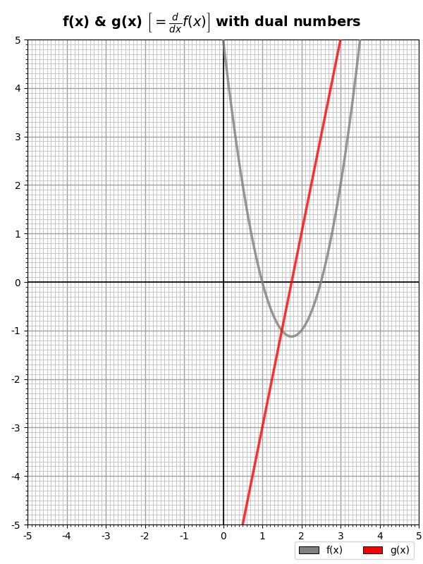
When run, this produces and saves dualnums-test.png:
As you see, the function takes a list of X-axis values and two lists of Y-axis values for two curves it presumes are a function, f(x), and its derivative, g(x).
The final step is putting it together and using dual numbers to generate the second list of data points (given the first one):
002| from traceback import extract_tb
003| from examples import kwarg, dualnumber, make_chart
004|
005| def main (**kwargs):
006| ”’Dual number demo.”’
007| fname = kwarg(‘fname’, ‘dualnums.png’, str, kwargs)
008| fpath = kwarg(‘fpath’, r’C:\Demo\HCC\Python’, str, kwargs)
009| poly = kwarg(‘poly’, ‘2, -7, 5’, str, kwargs)
010| xmin = kwarg(‘xmin’, –5.0, float, kwargs)
011| xmax = kwarg(‘xmax’, +5.0, float, kwargs)
012| ymin = kwarg(‘ymin’, –5.0, float, kwargs)
013| ymax = kwarg(‘ymax’, +5.0, float, kwargs)
014| xtix = kwarg(‘xtix’, ‘1.0, 0.1’, str, kwargs)
015| ytix = kwarg(‘ytix’, ‘1.0, 0.1’, str, kwargs)
016| divs = kwarg(‘divs’, 500, int, kwargs)
017|
018| coefficients = [float(n.strip()) for n in reversed(poly.split(‘,’))]
019|
020| def f (x):
021| accum = float()
022| for expon,coe in enumerate(coefficients):
023| accum += (coe * pow(x,expon))
024| return accum
025|
026| # Generate X-axis…
027| stepsize = (xmax–xmin)/divs
028| xs = [xmin+(ix*stepsize) for ix in range(divs)]
029|
030| # Generate data: f(x) and g(x)…
031| fys = [f(x) for x in xs]
032| gys = [dualnumber.differentiate(f,x) for x in xs]
033|
034| props = {
035| ‘fname’: fname, ‘fpath’:fpath,
036| ‘xmin’: xmin, ‘xmax’: xmax,
037| ‘ymin’: ymin, ‘ymax’: ymax,
038| ‘xticks’: tuple(float(n.strip()) for n in xtix.split(‘,’,1)),
039| ‘yticks’: tuple(float(n.strip()) for n in ytix.split(‘,’,1)),
040| }
041| make_chart(xs, fys,gys, **props)
042|
043| if __name__ == ‘__main__’:
044| print(argv[0])
045| print()
046|
047| # Convert commandline args to keyword args…
048| kwargs = {}
049| for arg in argv[1:]:
050| nam,val = arg.split(‘=’,1)
051| kwargs[nam] = val
052|
053| # Call main from inside a try/except…
054| try:
055| main(**kwargs)
056|
057| except:
058| # Print exception data in a nice, clear way…
059| etype, evalue, tb = exc_info()
060| ts = extract_tb(tb)
061| print()
062| print(f’{etype.__name__}: {evalue!s}‘)
063| print()
064| for t in ts[–5:]:
065| print(f’[{t[1]}] {t[2]} ({t[0]})‘)
066| print(f’ {t[3]}‘)
067| print()
068| print()
069| print()
070|
Lines #7 to #16 are like lines #12 to #21 in the make_chart function. They handle the keyword arguments (using the kwarg function). The poly argument is expected to be a comma-separated list of numbers which are taken as polynomial coefficients and applied like this:

So, for example, we express our function above, 2x² – 7x + 5, with the string “2, -7, 5”, which applies the 2 to the x² term, the -7 to the x¹ term, and 5 to the x⁰ term (remember, x⁰ is just 1). The string must include all coefficients, so if we wanted the function to be just x³, we’d pass “1,0,0,0” (for just x², pass”1,0,0″). Note that the poly argument has for a default “2,-7,5”.
Lines #18 to #24 implement this configurable polynomial function with the actual function defined starting in line #20.
Lines #26 to #32 generate the X-Y data starting with the list of x values. These are passed to the polynomial function to generate the function curve and to dualnumber.differentiate to generate the curve for the derivative.
Lines #34 to #40 create the keyword arguments for make_chart, passing along the xmin, xmax, ymin, and ymax input values (which control the range of the chart). The xticks and yticks parameters are derived from the xtix and ytix input arguments (which for convenience allow a comma-separated “min, max” string value).
Line #41 calls make_chart.
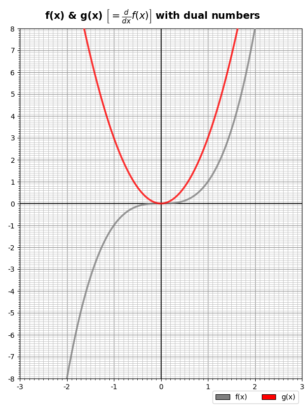
When run, it produces this chart:
Which is, indeed, the function 2x² – 7x + 5 and its derivative 4x – 7. And all we needed was the function itself and the dual numbers. Cool, eh?
Let’s end with something a little more interesting:
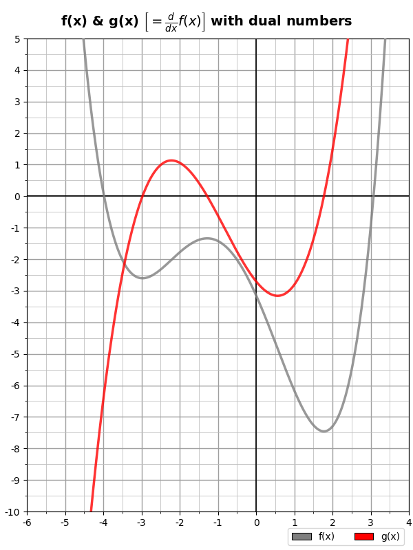
Which was created with the following parameters:
poly="0.1, 0.33, -0.75, -2.7, -3.1415",
xmin=-6, xmax=+4,
ymin=-10, ymax=+5,
xtix="1.0, 0.5", ytix="1.0, 0.5"
Which generates the function:

And its derivative:

Without breaking a sweat.
A very handy trick for your toolkit if you ever need to calculate a derivative from a set of data points (that were presumably generated by some function, but this technique should deliver good results even if not).
Below is a Desmos graph for the function:

And its derivative:

On the graph, these are respectively the red and purple lines. To emphasize the point, the purple line is the exact mathematical derivative of the red line.
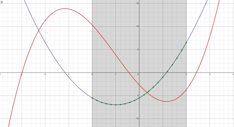
The green dots were calculated for the range -2 to +2 using dual numbers implemented by the code above. As you see, they lie precisely on the purple line.
Link: Zip file containing all code fragments used in this post.
∅

ATTENTION: The WordPress Reader strips the style information from posts, which can destroy certain important formatting elements. If you’re reading this in the Reader, I highly recommend (and urge) you to [A] stop using the Reader and [B] always read blog posts on their website.
This post is: Dual Numbers in Python
I often use the ForwardDiff library in Julia to use dual numbers, do you know if there is a similar library in python? I totally get the allure of implementing the class yourself but my student are often scared of switching language and not skilled enough to come with a good implementation themselves.
If you don’t know of one what would be the proper way for them to credit your code if they were to choose to use it?
I’ve never used them myself, but the PyPi site offers num-dual and dual-numbers.
You or your students can also use any online Ai to provide a nice working implementation in Python. I just got a nice one from the prompt to Copilot: “dual numbers in Python”.
No need to give credit if you use my code. If you want, a link to this post is fine.
Pingback: Dual Numbers and Why 0!=1 | Logos con carne